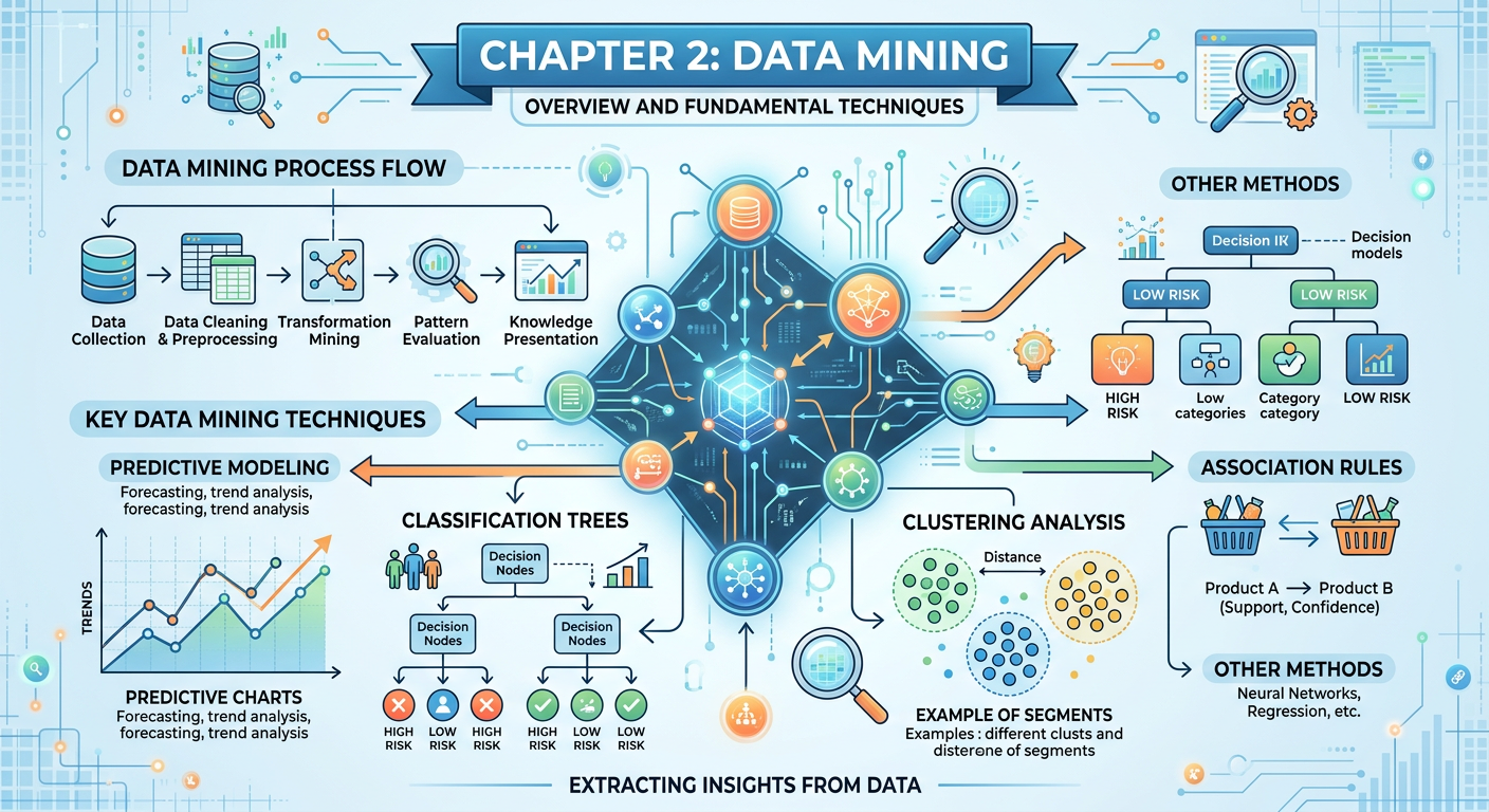
Figure 1:Explainer Infographic: Chapter 2: Data Mining.
1Introduction: Why Data Mining Matters in the Age of AI
Every time Amazon recommends a product you did not know you needed, every time your bank flags a suspicious transaction before you notice it yourself, and every time Netflix serves up a show that keeps you watching past midnight — data mining is at work. These are not accidents of technology. They are the deliberate results of algorithms trained on vast stores of behavioral, transactional, and contextual data to find patterns that human analysts could never surface on their own.
Data mining sits at the intersection of statistics, computer science, and business intelligence. For graduate students in business analytics, it is the discipline that converts raw organizational data into actionable competitive intelligence. Unlike simple reporting — which tells you what happened — data mining tells you why it happened, what will happen next, and which customers, products, or processes deserve your attention right now. In an era where generative AI tools can write code and summarize documents in seconds, the business analyst who understands the conceptual and strategic dimensions of data mining holds a profound advantage: you can direct AI tools intelligently, evaluate their outputs critically, and explain findings to executives who must act on them.
This chapter introduces the three foundational pillars of data mining as practiced in modern enterprise environments: predictive modeling, classification, and clustering. We will explore each concept from first principles, ground every idea in real-world business applications, and arm you with both vocabulary and intuition. By the end of this chapter, you should be able to select appropriate mining techniques for a given business problem, interpret model outputs with confidence, and use cutting-edge AI-powered tools — specifically Google’s NotebookLM — to deepen your analysis.
22.1 What Is Data Mining? Foundations and Framing
Data mining is the computational process of discovering patterns, anomalies, correlations, and actionable insights within large datasets using statistical and machine learning techniques. The term itself can be misleading: we are not mining for data — data is already abundant. We are mining within data for knowledge. The analogy most often cited in academic literature is that of gold mining: you move enormous amounts of rock (raw data) to find small but extraordinarily valuable nuggets (insights).
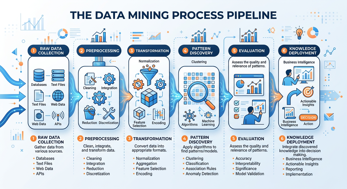
Figure 2:The Knowledge Discovery in Databases (KDD) Process — from raw data to actionable knowledge.
The broader framework within which data mining operates is called Knowledge Discovery in Databases (KDD), introduced by Fayyad, Piatetsky-Shapiro, and Smyth in their landmark 1996 paper. KDD is an iterative process that includes data selection, preprocessing, transformation, mining, and interpretation of results. Data mining is technically just one step in this pipeline, but it is the most computationally intensive and analytically rich stage, which is why the terms are often used interchangeably in practice.
2.12.1.1 Data Mining vs. Business Intelligence vs. Machine Learning
Graduate students frequently encounter confusion between data mining, business intelligence (BI), and machine learning (ML). These disciplines are related but distinct:
Business Intelligence focuses on historical reporting and dashboards. It answers questions like “What were our Q3 sales by region?” BI tools include Tableau, Power BI, and Looker. BI is descriptive and diagnostic.
Data Mining goes further by discovering non-obvious patterns in historical and current data. It is predictive and prescriptive, revealing relationships that analysts did not know to look for.
Machine Learning is the set of algorithmic techniques that often power data mining. Where data mining is a goal (find patterns), machine learning is a method (train models on data to recognize patterns automatically).
In contemporary usage, especially in an AI-augmented enterprise, these three domains have become deeply intertwined. A modern analytics platform like Salesforce Einstein or AWS SageMaker integrates all three seamlessly. Understanding their distinctions, however, helps you select the right tool for the right business question.
2.22.1.2 The CRISP-DM Framework
The Cross-Industry Standard Process for Data Mining (CRISP-DM) is the most widely adopted methodology for structuring data mining projects in industry. Originally published in 1999 by a consortium including IBM, SPSS, and NCR, CRISP-DM defines six iterative phases:
Business Understanding — Articulate the business problem, define success criteria, and translate objectives into a data mining problem statement.
Data Understanding — Collect initial data, explore it, identify quality issues, and discover first insights.
Data Preparation — Select, clean, construct, integrate, and format data for modeling.
Modeling — Select and apply modeling techniques, calibrate parameters, and build models.
Evaluation — Assess whether models genuinely meet business objectives; review the process before deployment.
Deployment — Deliver results: from a simple written report to a fully automated scoring pipeline integrated into a CRM system.
The arrows in the CRISP-DM diagram are bidirectional because real projects are iterative. You frequently discover during modeling that your data preparation was insufficient and must backtrack. A senior analytics manager at a Fortune 500 company once told the author: “We spend 80% of our time in phases two and three, and only 20% on the glamorous modeling work.” This is an important reality check for students who are drawn to the algorithmic excitement of machine learning without appreciating the critical importance of clean, well-understood data.
32.2 Predictive Modeling: Forecasting Business Outcomes
Predictive modeling is the practice of using historical data and statistical algorithms to estimate future outcomes. It answers questions like: “Which customers are most likely to churn next quarter?” “What is the probability that this loan applicant will default?” “How much revenue will we generate in Q4 if current trends continue?” These are not hypothetical academic exercises — they are questions that drive billions of dollars in business decisions every year.
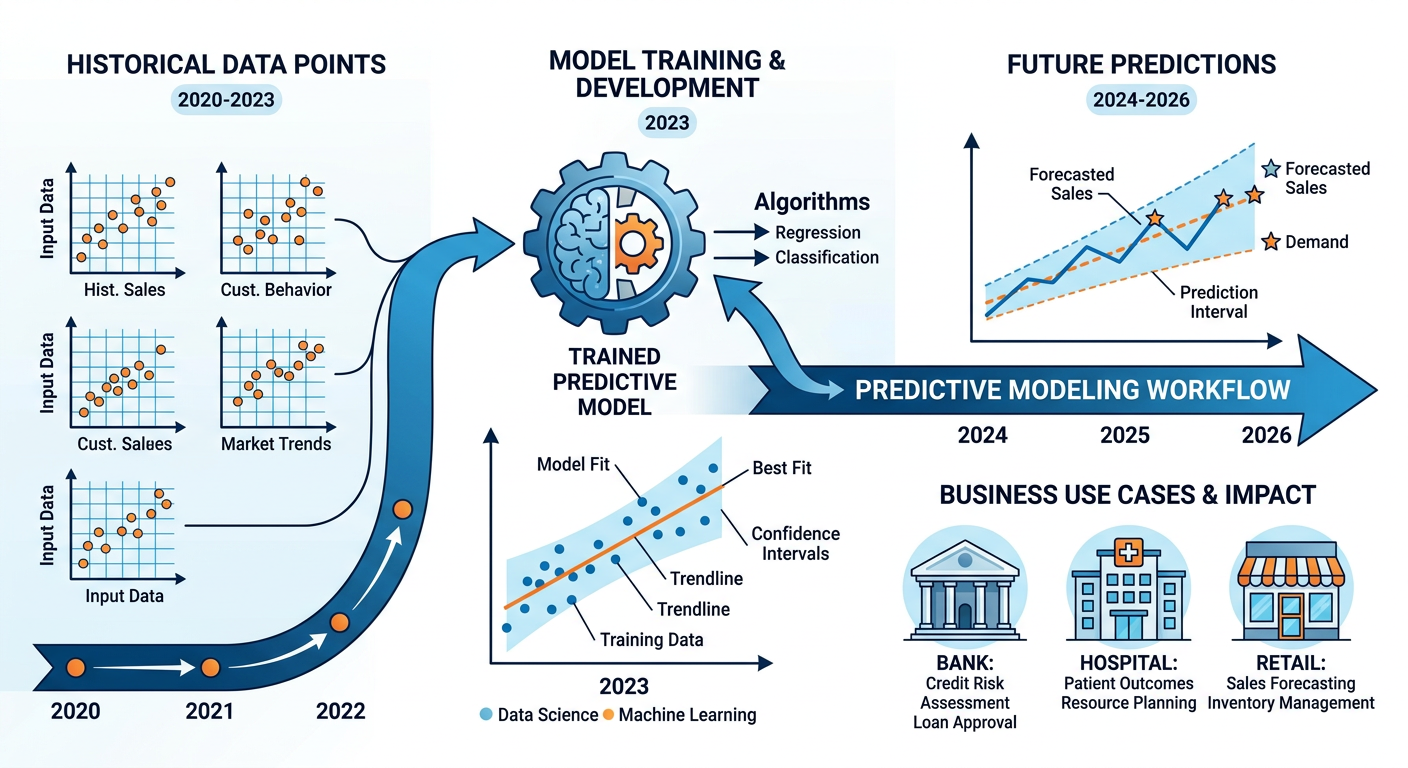
Figure 3:Predictive Modeling Workflow: From historical data to business forecasts.
3.12.2.1 The Architecture of a Predictive Model
Every predictive model shares a common architectural logic. You have a target variable (also called a dependent variable or outcome) — the thing you want to predict. You have predictor variables (also called features or independent variables) — the observable characteristics of each case that you believe relate to the target. The model learns the mathematical relationship between predictors and the target during a training phase using historical cases where both predictors and outcomes are known. It then applies that learned relationship to new cases where only the predictors are available.
For example, a bank building a loan default prediction model might define:
Target variable: Default within 12 months (Yes/No)
Predictor variables: Credit score, debt-to-income ratio, employment history, loan amount, loan purpose, prior delinquencies, etc.
The model trains on thousands of past loan records and learns that, say, a debt-to-income ratio above 43% combined with fewer than two years of employment history dramatically increases default risk. It then scores incoming loan applications with those features to produce a probability estimate — for instance, “This applicant has a 34% probability of defaulting.” The loan officer can now make a more informed decision than gut instinct alone would allow.
3.22.2.2 Regression: The Classic Predictive Engine
Linear regression is the foundational technique for predicting continuous outcomes. Despite its age — the method dates to Gauss and Legendre in the early nineteenth century — linear regression remains extraordinarily powerful and widely deployed in business. It models the relationship between a continuous target variable and one or more predictors as a linear equation:
Where is the predicted value, is the intercept, through are coefficients learned from data, and is the error term. The coefficients represent the marginal effect of each predictor: a one-unit increase in , holding all else constant, is associated with a -unit change in .
In a business context, a retail company might build a linear regression model predicting weekly store revenue () as a function of local population density, median household income, square footage of the store, number of competitors within five miles, and promotional spend. The resulting model can be used to forecast revenue for new store locations under consideration, enabling data-driven site selection.
Logistic regression extends this framework to binary outcomes — situations where the target variable is categorical rather than continuous (e.g., “Will this customer click the ad? Yes or No?”). Rather than predicting a raw value, logistic regression predicts the probability that an observation belongs to a particular category, constrained between 0 and 1 using the logistic (sigmoid) function. We will revisit logistic regression in the classification section, as it is one of the most important tools in the business analyst’s toolkit.
3.32.2.3 Overfitting and Generalization: The Central Challenge
One of the most important concepts in predictive modeling — and one that students frequently underestimate — is overfitting. A model that is too complex can memorize the training data perfectly, including all its noise and quirks, but perform terribly on new, unseen data. This is analogous to a student who memorizes every practice exam question verbatim but cannot answer a slightly different question on the actual test. The model has learned the training data, not the underlying pattern.
The antidote to overfitting is generalization — the ability of a model to perform well on data it has never seen. Business analysts achieve this through several strategies:
Train/Test Split: Reserve a portion of labeled data (typically 20–30%) as a hold-out test set that is never used during training. After training, evaluate model performance on this unseen set to estimate real-world accuracy.
Cross-Validation: Divide data into folds; train on folds and test on the remaining fold, rotating through all combinations. Average performance across all folds for a robust estimate.
Regularization: Techniques like Ridge (L2) and Lasso (L1) regression penalize overly complex models by shrinking coefficients toward zero, reducing overfitting.
42.3 Classification: Sorting the World into Actionable Categories
Classification is a type of supervised learning in which the goal is to assign each observation to one of a finite set of predefined categories based on its features. It is perhaps the most practically versatile branch of data mining, with applications spanning virtually every industry. Credit scoring, disease diagnosis, email spam filtering, fraud detection, customer segmentation by purchase intent, image recognition in retail environments — all of these are classification problems at their core.
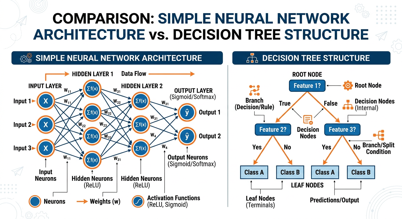
Figure 4:Three Core Classification Approaches: Decision Trees, Logistic Regression, and Random Forests.
The key distinction from regression is the nature of the target variable: in regression, we predict a continuous number; in classification, we predict a discrete label or category. When there are exactly two categories (e.g., fraud vs. not fraud), we call it binary classification. When there are three or more categories (e.g., classifying customer service inquiries as billing, technical support, returns, or general inquiry), we call it multi-class classification.
4.12.3.1 Decision Trees: Interpretable Intelligence
Decision trees are among the most intuitive and interpretable classification algorithms available. They model a classification problem as a series of hierarchical if-then-else rules, creating a tree structure in which:
Each internal node represents a test on a feature (e.g., “Is the transaction amount greater than $500?”)
Each branch represents the outcome of that test
Each leaf node represents a class label or prediction
Decision trees are learned from data by recursively splitting the dataset on the feature that best separates the classes at each step. The most common splitting criteria are Gini impurity and Information Gain (entropy). Gini impurity measures the probability that a randomly chosen element would be incorrectly classified if it were randomly labeled according to the distribution in the node. Information Gain measures the reduction in entropy — or disorder — achieved by a given split.
Consider a credit card company building a fraud detection system. The decision tree might learn:
If transaction amount > $2,000 → proceed
If merchant category = “Electronics” → check further
If transaction is outside the cardholder’s home country → FLAG AS FRAUD (probability: 0.87)
If transaction is domestic → Not Fraud (probability: 0.93)
If merchant category ≠ “Electronics” → Not Fraud (probability: 0.78)
If transaction amount ≤ $2,000 → Not Fraud (probability: 0.95)
This is, of course, a simplified illustration. Real fraud detection trees have hundreds of nodes and consider dozens of features. But the logic is transparent, auditable, and explainable to a regulatory body — which is a significant advantage in regulated industries.
The chief weakness of decision trees is their instability: a small change in the training data can produce a dramatically different tree. They are also prone to overfitting when grown too deep. These weaknesses motivate ensemble methods.
4.22.3.2 Random Forests: The Power of Collective Intelligence
**A ** random forest is an ensemble of many decision trees, each trained on a random bootstrap sample of the training data and using a random subset of features at each split. The final prediction is determined by majority vote (for classification) or averaging (for regression) across all trees. This elegant approach leverages two statistical principles: bagging (bootstrap aggregating) reduces variance by averaging across diverse models, and feature randomization further decorrelates the individual trees, making the ensemble more robust.
Random forests consistently deliver exceptional performance across a wide range of business problems. They are highly resistant to overfitting, handle missing data well, are relatively immune to outliers, and require minimal data preprocessing (no need to scale features, for instance). Their primary limitation is interpretability: while you can extract feature importance rankings from a random forest, explaining why a specific prediction was made is far more difficult than with a single decision tree. This creates tension in contexts where explainability is a regulatory requirement — for example, under the Equal Credit Opportunity Act, lenders must be able to explain adverse actions taken against credit applicants.
4.32.3.3 Logistic Regression as a Classifier
While we introduced logistic regression in the predictive modeling section, it is critical to understand its role as a classifier. Logistic regression does not just predict a probability — it can be used to make a binary classification decision by applying a decision threshold (typically 0.5): observations with predicted probability ≥ 0.5 are assigned to class 1 (e.g., “churn”), while those with predicted probability < 0.5 are assigned to class 0 (e.g., “no churn”).
Logistic regression is prized for its interpretability. The coefficients, when exponentiated, become odds ratios with direct business meaning. In a churn prediction model, a coefficient of 0.69 for the variable “number of support calls in the last 90 days” yields an odds ratio of , meaning each additional support call doubles the odds of churning. This is actionable intelligence: the retention team should prioritize outreach to customers with high support call frequencies.
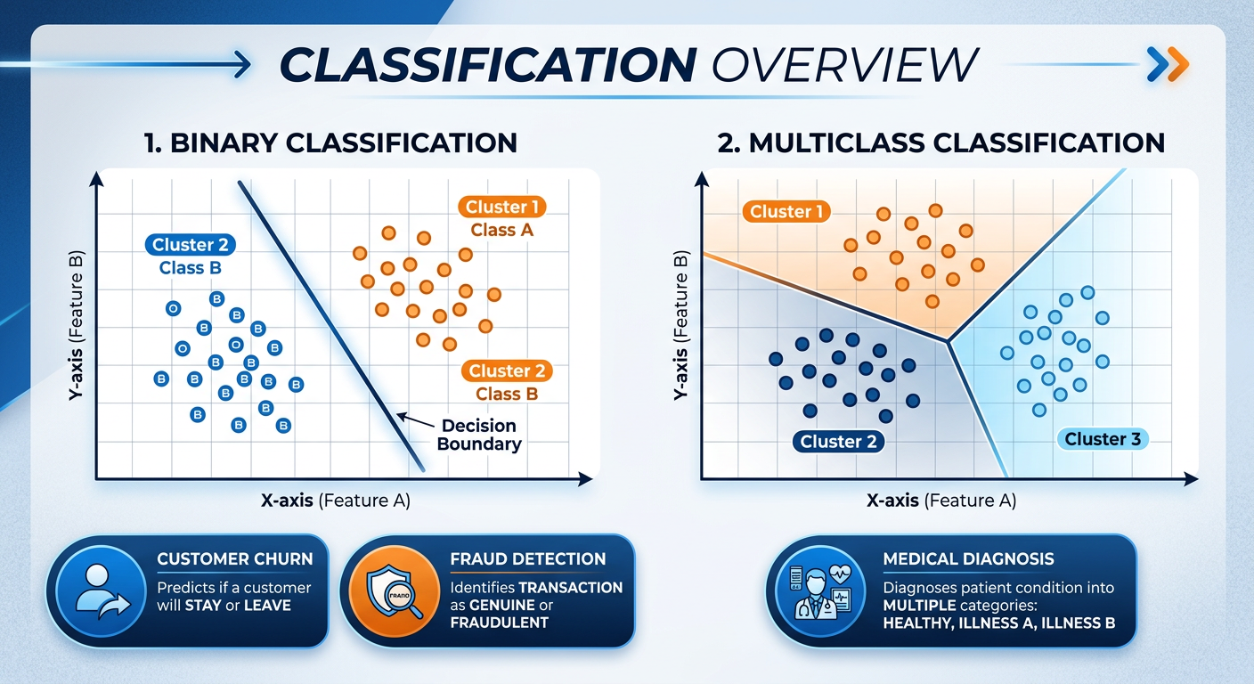
Figure 5:Classification Performance Metrics: Confusion Matrix, Precision, Recall, F1-Score, and ROC-AUC.
4.42.3.4 Evaluating Classification Models
Model accuracy — the proportion of correctly classified cases — is the most intuitive performance metric, but it can be deeply misleading in business contexts characterized by class imbalance. Consider a fraud detection scenario where only 0.5% of all transactions are fraudulent. A model that simply predicts “not fraud” for every single transaction achieves 99.5% accuracy while being completely useless. More meaningful metrics include:
Precision: Of all cases predicted as positive (fraud), what proportion are actually positive? High precision means few false alarms.
Recall (Sensitivity): Of all actual positive cases, what proportion did the model correctly identify? High recall means fewer missed frauds.
F1-Score: The harmonic mean of Precision and Recall — a single metric that balances both concerns.
ROC-AUC: The Area Under the Receiver Operating Characteristic Curve measures the model’s ability to discriminate between classes across all possible decision thresholds. An AUC of 1.0 is a perfect classifier; 0.5 is no better than random chance. For most business applications, an AUC above 0.80 is considered acceptable, above 0.90 excellent.
The business context determines which metric matters most. A cancer screening test should maximize recall (missing a cancer is far more costly than a false alarm that triggers a follow-up test). A spam filter should maximize precision (wrongly blocking a legitimate business email may be more costly than letting some spam through). Business analysts must engage with domain experts to align metric choices with real-world cost structures.
Primary Concern: Missing actual fraud (false negatives) is very costly — the company absorbs the loss. Key Metric: Recall — maximize the proportion of actual fraud cases caught. Trade-off accepted: Some false alarms (flagging legitimate transactions) is acceptable if it catches more fraud.
Primary Concern: Approving loans that will default (false positives) destroys profitability. Key Metric: Precision — ensure that approved loans are truly creditworthy. Trade-off accepted: Some creditworthy applicants may be rejected if the model is conservative.
Primary Concern: Missing positive cases has life-or-death consequences. Key Metric: Recall (Sensitivity) — catch as many true positives as possible. Trade-off accepted: High false positive rate leading to unnecessary follow-up testing.
Primary Concern: Blocking important legitimate emails (false positives) disrupts business. Key Metric: Precision — ensure flagged emails are genuinely spam. Trade-off accepted: Some spam may reach the inbox if the filter is conservative.
52.4 Clustering: Discovering Natural Structure in Data
Clustering belongs to the family of unsupervised learning methods — techniques applied when we do not have labeled training data and instead want the algorithm to discover natural groupings or structure within the data on its own. Unlike classification, there is no predefined target variable. The algorithm must infer the “correct” groups from the patterns and distances among observations.
The business motivation for clustering is profound. Before you can personalize marketing messages, you must first understand that your customer base is not homogeneous — it consists of distinct behavioral segments with different needs, values, and response patterns. Before you can optimize a supply chain, you must identify which products cluster together in demand patterns. Before you can prioritize IT security monitoring, you must identify which servers cluster into normal behavioral profiles so that anomalous behavior stands out.
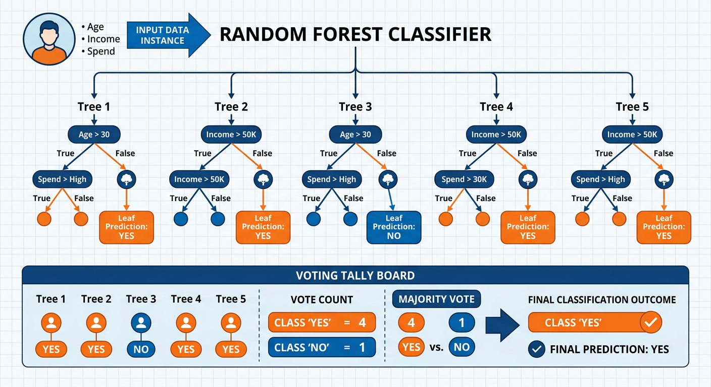
Figure 6:K-Means Clustering: Iterative centroid assignment and recalculation until convergence.
5.12.4.1 K-Means Clustering: Simple, Powerful, Pervasive
K-means is the most widely deployed clustering algorithm in business settings, valued for its computational efficiency and conceptual simplicity. The algorithm operates as follows:
Initialize: Randomly select data points as initial cluster centroids.
Assign: Assign each observation to the nearest centroid based on Euclidean distance (or another distance measure).
Update: Recalculate each centroid as the mean of all observations currently assigned to that cluster.
Repeat: Iterate steps 2 and 3 until cluster assignments no longer change (convergence).
The result is clusters, each defined by its centroid — the average position of its members in feature space.
Selecting : The analyst must specify the number of clusters before running the algorithm, which raises the practical question: how many clusters is “right”? Several techniques help:
The Elbow Method: Plot the total within-cluster sum of squares (WCSS) against various values of . WCSS decreases as increases (more clusters = smaller, tighter groups). Look for the “elbow” — the point of diminishing returns where adding another cluster yields minimal reduction in WCSS.
Silhouette Analysis: Measures how similar each point is to its own cluster compared to other clusters. Silhouette scores range from -1 to +1; higher scores indicate better-defined clusters.
Business Heuristics: Sometimes the number of clusters is driven by practical constraints — a marketing team that can execute three distinct campaign strategies effectively should not build a six-segment model they cannot act on.
5.22.4.2 A Real-World K-Means Application: Retail Customer Segmentation
Consider a regional grocery chain with loyalty card data on 500,000 customers. The data science team extracts behavioral features for each customer over the past 12 months: total spend, number of visits per month, average basket size, proportion of spend on private-label products, proportion of spend on fresh produce, proportion of spend on health and wellness products, and recency of last visit.
Running k-means with might reveal segments like:
| Segment | Description | Strategy |
|---|---|---|
| 1 | High-frequency, health-conscious shoppers | Premium organic promotions, wellness newsletter |
| 2 | Budget-focused families, high private-label purchase | Value bundles, BOGO promotions |
| 3 | Occasional shoppers, high basket size when they visit | Re-engagement campaigns, delivery offers |
| 4 | Fresh produce devotees, low packaged goods spend | Farm-to-table content, local sourcing messaging |
| 5 | Lapsed customers, declining visit frequency | Win-back offers, personalized discounts |
Each segment calls for a fundamentally different marketing and retention strategy. Without clustering, the chain might have sent the same promotional email to all 500,000 customers — a spray-and-pray approach that generates low response rates and wastes marketing budget. With clustering, it can deliver precisely targeted communications that resonate with each group’s actual behavior and preferences.
5.32.4.3 Hierarchical Clustering: When You Do Not Know 
Hierarchical clustering offers an alternative to k-means that does not require pre-specifying the number of clusters. It builds a hierarchy of clusters in one of two ways:
Agglomerative (bottom-up): Begin with each observation as its own cluster. Repeatedly merge the two closest clusters until all observations belong to one cluster. This is the more common approach.
Divisive (top-down): Begin with all observations in one cluster. Repeatedly split the least cohesive cluster until each observation is its own cluster.
The output is a dendrogram — a tree-like diagram that illustrates the merging sequence and the distances at which merges occurred. Analysts can “cut” the dendrogram at different heights to produce different numbers of clusters, which makes it an exploratory tool for understanding natural data structure.
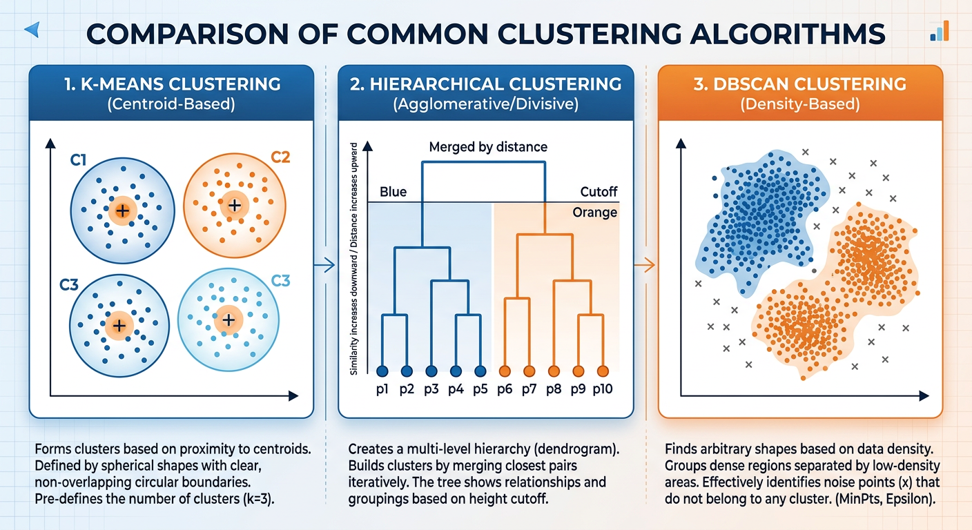
Figure 7:Hierarchical Clustering Dendrogram: Cutting at different heights yields different cluster solutions.
Hierarchical clustering is computationally expensive — its time complexity is O(n²), making it impractical for very large datasets. However, for datasets of moderate size (say, up to 10,000 observations), it provides invaluable exploratory insight. It is particularly popular in bioinformatics (clustering gene expression patterns), marketing research (segmenting survey respondents), and competitive intelligence (grouping competitor products by feature similarity).
5.42.4.4 DBSCAN: Clustering by Density
Density-Based Spatial Clustering of Applications with Noise (DBSCAN) takes an entirely different approach to clustering. Rather than minimizing distance to centroids, DBSCAN identifies clusters as dense regions of observations separated by regions of low density. It requires two parameters: epsilon (ε), the maximum distance between two points for them to be considered neighbors, and MinPts, the minimum number of points required to form a dense region.
DBSCAN offers two key advantages over k-means: (1) it can discover clusters of arbitrary shape — not just spherical clusters — and (2) it explicitly handles noise points (outliers) that do not belong to any cluster, labeling them as such rather than forcing them into the nearest cluster. This makes DBSCAN particularly valuable for anomaly detection, geographic clustering of customer locations (urban clusters are not spherical), and any domain where noise is expected.
62.5 Advanced Topics: The Modern Data Mining Landscape
6.12.5.1 Association Rule Mining: The Market Basket Problem
Association rule mining discovers interesting relationships between variables in large transaction databases. It is the algorithm behind the famous “beer and diapers” story (whether apocryphal or not) and countless real-world retail discoveries. The classic formulation is the Market Basket Analysis problem: given a database of retail transactions, find rules of the form “Customers who buy items A and B also tend to buy item C.”
Rules are evaluated by three metrics:
Support: The proportion of transactions containing all items in the rule. Low support means the pattern is rare and may not be business-relevant.
Confidence: Given that a customer bought items A and B, the probability they also bought C. Higher confidence means the rule is more reliable.
Lift: The ratio of confidence to the baseline probability of buying C. Lift > 1 indicates a genuine positive association beyond what would be expected by chance.
The Apriori algorithm and its more efficient successors (FP-Growth) make it computationally feasible to search through exponentially large rule spaces. In e-commerce, association rules power recommendation engines, complementary product suggestions, and cross-sell campaigns. Streaming services use similar logic (collaborative filtering) to recommend content based on viewing patterns shared across similar users.
6.22.5.2 Time Series Forecasting as Predictive Mining
Many business data mining problems are inherently temporal — sales data, website traffic, stock prices, and energy consumption all unfold over time. Time series forecasting is a specialized form of predictive modeling that accounts for temporal structure: trends, seasonality, cycles, and autocorrelation (the tendency of a value to be correlated with its own past values).
Classical approaches include ARIMA (AutoRegressive Integrated Moving Average) models. Modern approaches leverage machine learning — gradient boosted trees with engineered time features, or recurrent neural networks (RNNs) and Long Short-Term Memory (LSTM) networks for deep learning-based forecasting. Meta’s open-source Prophet library, designed for business forecasting with strong seasonality and holiday effects, has become widely adopted in industry for its accessibility and robustness.
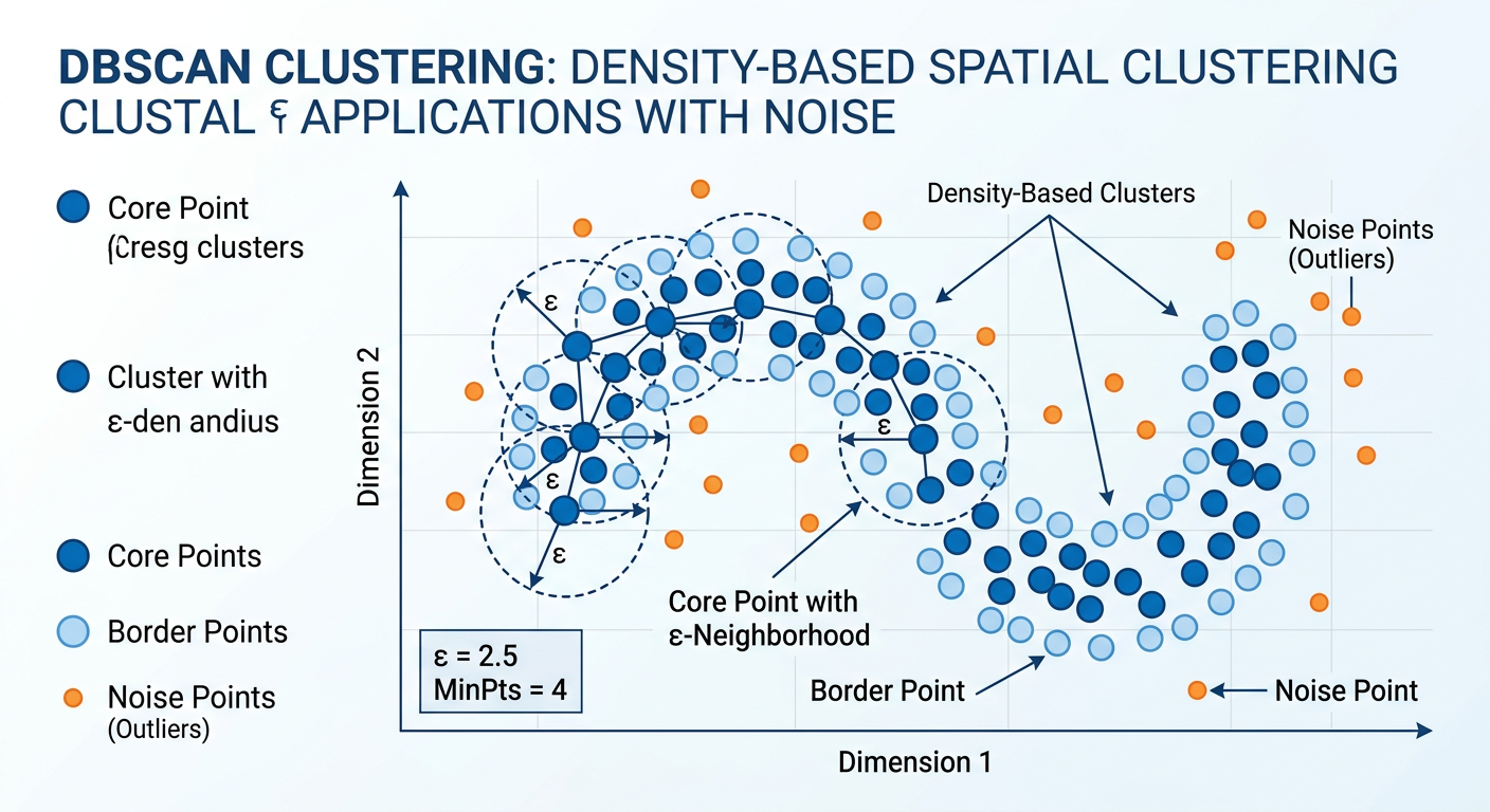
Figure 8:Time Series Forecasting: Decomposing trend and seasonality to project future business outcomes.
6.32.5.3 Data Mining in the Age of Generative AI
The rise of large language models (LLMs) like GPT-4o/o3 (OpenAI), Claude Sonnet 4.5 (Anthropic), and Gemini 2.0 (Google) has fundamentally transformed the data mining landscape. By 2025–2026, these models serve not just as text generators but as reasoning partners capable of designing entire data mining workflows, writing and debugging code, and interpreting complex model outputs for non-technical stakeholders. These models represent a new form of “pattern mining” — trained on vast corpora of text data to learn language structure, world knowledge, and reasoning patterns — but they also serve as powerful tools for supporting traditional data mining workflows.
Business analysts now use LLMs to:
Generate and explain code: Write Python or R scripts for data preprocessing, modeling, and visualization, then explain what the code does.
Interpret model outputs: Translate complex statistical results into plain-language business narratives.
Accelerate literature review: Summarize academic papers on advanced modeling techniques.
Augment qualitative analysis: Analyze open-ended customer survey responses, social media sentiment, and support ticket text at scale using natural language processing.
72.6 Integrating Data Mining into Business Strategy
Data mining does not exist in a vacuum. Its value is realized only when mining outputs are connected to decisions, processes, and strategies that organizations can actually execute. This section bridges the technical world of algorithms and models with the practical world of business operations, change management, and competitive strategy.
7.12.6.1 From Model to Decision: The Deployment Challenge
Building a predictive model that performs well on a test dataset is, in many organizations, the easiest part of the data mining journey. The harder challenge is deployment: integrating the model into live business systems so that its predictions influence real decisions in real time. Consider the difference between:
A churn prediction model that a data scientist runs manually in a Jupyter notebook once per quarter and emails results to the marketing team as a spreadsheet attachment.
A churn prediction model embedded in the company’s CRM system that automatically scores every customer daily, triggers personalized retention offers via email for high-risk customers, and logs all interventions and outcomes for continuous model retraining.
The first scenario delivers some value; the second delivers transformational value. The gap between them involves engineering work, organizational processes, stakeholder alignment, and governance frameworks — none of which are purely technical challenges. According to Gartner research, only about 54% of AI and data science projects successfully transition from pilot to production — a figure that has remained stubbornly persistent despite improvements in MLOps tooling. A 2024 McKinsey survey found that while 78% of organizations report using AI in at least one business function, only a minority have achieved enterprise-wide deployment with measurable ROI. Understanding this deployment gap is essential for any business analytics professional who aspires to drive real organizational impact.
7.22.6.2 Model Governance and the Ethical Dimension
As data mining models become embedded in high-stakes business decisions — who gets credit, who gets hired, who receives medical treatment — the ethical and governance dimensions become impossible to ignore. Model governance refers to the organizational policies, processes, and oversight mechanisms that ensure models are accurate, fair, transparent, and compliant with applicable regulations.
Key governance concerns include:
Bias and Fairness: Training data reflects historical human decisions, which may themselves embed discrimination. A hiring algorithm trained on historical promotion data may learn to penalize characteristics associated with underrepresented groups, not because those characteristics are actually predictive of job performance, but because historical promotion rates were biased. Analysts must audit models for disparate impact across protected classes.
Data Privacy: Mining customer data raises significant privacy concerns. In the United States, sector-specific regulations (HIPAA for health data, FERPA for education data, GLBA for financial data) impose strict constraints. The California Consumer Privacy Act (CCPA) and the EU’s GDPR add further layers. Business analysts must understand the data governance frameworks within which they operate.
Model Drift: The world changes, and models trained on historical data can become stale. A credit scoring model trained before the COVID-19 pandemic may perform poorly on post-pandemic credit behavior. Organizations need systematic model monitoring processes that detect performance degradation and trigger retraining when necessary.
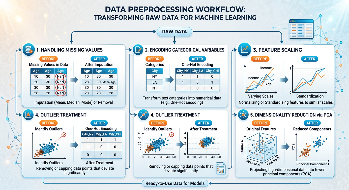
Figure 9:Data Mining Model Governance: A continuous cycle from development to refresh.
7.32.6.3 Competitive Advantage Through Data Mining
Organizations that develop mature data mining capabilities build durable competitive advantages that are genuinely difficult for rivals to replicate. This is because the competitive moat is not the algorithm — most algorithms are freely available in open-source libraries — but the proprietary data assets, the organizational learning embedded in refined data pipelines, and the talent and culture that enable continuous improvement.
Amazon’s recommendation engine is not valuable because Amazon invented collaborative filtering — the algorithm is decades old and publicly documented. It is valuable because Amazon has accumulated transaction data on hundreds of millions of customers over three decades, and it has built an organizational culture and technical infrastructure that continuously learns from every customer interaction. This data flywheel — where better data enables better models, which drive better customer experiences, which generate more data — is the fundamental mechanism of competitive advantage in the AI era.
For graduate business analytics students, the strategic implication is clear: data mining is not a one-time project. It is an organizational capability that must be built, maintained, and continuously evolved. Companies that treat analytics as an ongoing strategic function — not a periodic IT initiative — consistently outperform their competitors on key financial metrics. A 2021 McKinsey survey found that companies in the top quartile of data and analytics maturity were 23 times more likely to acquire customers, six times more likely to retain them, and 19 times more likely to be profitable than their least mature peers.
82.7 Practical Tools and Technologies
The data mining landscape is supported by a rich ecosystem of tools and platforms that have democratized access to sophisticated analytical techniques. Business analysts today can execute complex mining workflows without writing a single line of code — though coding fluency remains a powerful differentiator.
8.12.7.1 Python and R: The Analyst’s Workbench
Python and R are the two dominant programming languages for data mining in professional and academic settings. Python, with its extensive ecosystem of libraries — scikit-learn for machine learning, pandas for data manipulation, matplotlib and seaborn for visualization, statsmodels for statistical modeling, and XGBoost and LightGBM for gradient boosting — has become the de facto standard in industry. R, with its deep statistical heritage and packages like caret, randomForest, e1071, and the tidyverse, remains the preferred environment in academic research and certain industry verticals like pharmaceuticals and finance.
# Example: Building a Random Forest Classifier in Python
# Customer churn prediction using scikit-learn

import pandas as pd
from sklearn.model_selection import train_test_split
from sklearn.ensemble import RandomForestClassifier
from sklearn.metrics import classification_report, roc_auc_score
from sklearn.preprocessing import StandardScaler

# Load and prepare data
df = pd.read_csv('customer_data.csv')

# Define features and target
features = ['tenure_months', 'monthly_charges', 'num_support_calls',
            'num_products', 'has_contract', 'avg_monthly_usage']
X = df[features]
y = df['churned']  # Binary: 1 = churned, 0 = retained

# Train/test split (80/20)
X_train, X_test, y_train, y_test = train_test_split(
    X, y, test_size=0.2, random_state=42, stratify=y
)

# Train Random Forest
rf_model = RandomForestClassifier(
    n_estimators=200,
    max_depth=10,
    min_samples_leaf=5,
    random_state=42,
    class_weight='balanced'  # Handles class imbalance
)
rf_model.fit(X_train, y_train)

# Evaluate
y_pred = rf_model.predict(X_test)
y_prob = rf_model.predict_proba(X_test)[:, 1]

print(classification_report(y_test, y_pred))
print(f"ROC-AUC Score: {roc_auc_score(y_test, y_prob):.4f}")

# Feature Importance
importance_df = pd.DataFrame({
    'Feature': features,
    'Importance': rf_model.feature_importances_
}).sort_values('Importance', ascending=False)

print("\nFeature Importances:")
print(importance_df)
# Example: K-Means Customer Segmentation
import pandas as pd
import numpy as np
from sklearn.cluster import KMeans
from sklearn.preprocessing import StandardScaler
import matplotlib.pyplot as plt
# Load customer behavioral data
df = pd.read_csv('customer_behavior.csv')
# Select clustering features
cluster_features = ['total_spend', 'visit_frequency',
'avg_basket_size', 'recency_days']
X = df[cluster_features]
# Scale features (critical for distance-based algorithms)
scaler = StandardScaler()
X_scaled = scaler.fit_transform(X)
# Elbow method to select k
inertia = []
k_range = range(2, 11)
for k in k_range:
km = KMeans(n_clusters=k, random_state=42, n_init=10)
km.fit(X_scaled)
inertia.append(km.inertia_)
# Plot elbow curve
plt.figure(figsize=(8, 5))
plt.plot(k_range, inertia, marker='o', color='#1a73e8', linewidth=2)
plt.xlabel('Number of Clusters (k)', fontsize=12)
plt.ylabel('Within-Cluster Sum of Squares', fontsize=12)
plt.title('Elbow Method for Optimal k', fontsize=14)
plt.axvline(x=5, color='#ff6d00', linestyle='--', label='Selected k=5')
plt.legend()
plt.tight_layout()
plt.savefig('elbow_curve.png', dpi=150)
plt.show()
# Fit final model with selected k
final_km = KMeans(n_clusters=5, random_state=42, n_init=10)
df['Segment'] = final_km.fit_predict(X_scaled)
# Profile each segment
segment_profile = df.groupby('Segment')[cluster_features].mean()
print("Cluster Profiles:")
print(segment_profile.round(2))8.22.7.2 No-Code and Low-Code Platforms
Not every business analytics professional writes Python daily. Enterprise platforms like SAS Viya, IBM Watson Studio, Microsoft Azure Machine Learning, Google Vertex AI, and RapidMiner provide graphical, drag-and-drop interfaces for building and deploying data mining workflows. These platforms lower the barrier to entry and accelerate time-to-insight for business analysts who may not have deep programming backgrounds but need to apply data mining to real problems quickly.
The emergence of AutoML (Automated Machine Learning) tools — including Google AutoML, H2O.ai Driverless AI, and DataRobot — pushes this democratization even further. These systems automate feature engineering, model selection, hyperparameter tuning, and performance evaluation, producing deployment-ready models with minimal human intervention. The business analyst’s role in an AutoML world shifts from hands-on modeling to problem framing, data quality oversight, results interpretation, and stakeholder communication.
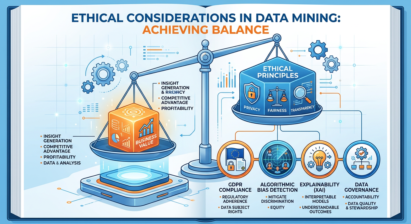
Figure 10:The Data Mining Technology Stack: From programming languages to AutoML platforms.
92.8 Discussion Question: The Netflix Recommendation Engine Case
9.1Case Background
Netflix operates one of the most studied and celebrated data mining systems in the world. With over 260 million paid subscribers across 190 countries, Netflix generates approximately 80% of viewer activity through its recommendation engine — meaning that 80% of what people watch is discovered through algorithmic suggestion rather than direct search. The system processes billions of data points daily: what users watch, for how long, when they pause, when they rewind, what they watch next, what they abandon, what device they are using, and even what artwork thumbnails they click on.
Netflix employs a sophisticated ensemble of data mining techniques: collaborative filtering (which finds users with similar taste profiles and recommends what similar users enjoyed), content-based filtering (which recommends content similar to what a user has previously liked, based on genre, director, cast, and thematic features), and contextual bandits (a reinforcement learning technique that personalizes thumbnail artwork — literally showing different images for the same show to different users based on predicted click-through probability).
In 2009, Netflix famously awarded the Netflix Prize — a $1 million competition — to a team that improved its recommendation algorithm’s accuracy by more than 10% on the RMSE (Root Mean Squared Error) metric. The winning solution was a massive ensemble of over 100 individual models. Strikingly, Netflix ultimately did not deploy the winning solution in production because the engineering complexity required to run it at scale was not justified by the marginal improvement in business outcomes relative to their existing system.
9.2Discussion Questions
Carefully read the case background above and reflect on the following questions. You are encouraged to conduct additional research using academic sources, the Netflix Technology Blog (netflixtechblog.com), and the resources you will explore in the Hands-On Activity using NotebookLM.
Algorithm vs. Business Value: The Netflix Prize-winning algorithm improved RMSE by over 10% but was not deployed because operational complexity outweighed business benefit. What does this teach us about the relationship between model performance metrics and real-world business value? How should organizations define “success” for a data mining project?
Data as Competitive Advantage: Netflix’s recommendation system derives much of its power not from proprietary algorithms (collaborative filtering is decades old and open source) but from the proprietary behavioral data it has accumulated. Do you agree that data is a more durable competitive advantage than algorithmic sophistication in the modern AI landscape? What are the counterarguments? Use specific examples from other industries to support your position.
Ethical Dimensions of Recommendation Systems: Netflix’s recommendation engine is designed to maximize engagement — keeping users watching as long as possible. Critics argue that engagement-maximizing algorithms can create “filter bubbles” (exposing users only to content that confirms existing preferences), promote binge-watching behaviors that may have negative psychological consequences, and systematically underexpose diverse or challenging content in favor of algorithmically “safe” mainstream choices. As a business analytics professional, how do you reconcile the business imperative to optimize engagement with broader ethical responsibilities to users and society?
Generalization to Your Domain: Identify a specific industry context relevant to your professional background or career aspirations (healthcare, finance, retail, logistics, public sector, etc.). Describe a recommendation or personalization system that could be built using the data mining techniques covered in this chapter. What data would you need? Which techniques would you apply? What ethical guardrails would you put in place?
9.3📝 Discussion Guidelines
Primary Response: Your initial post must address all parts of the prompt with depth and critical thinking. It must include at least one citation (scholarly or credible industry source) to support your argument.
Peer Responses: You must respond thoughtfully to at least two of your peers. Your responses must go beyond simple agreement (e.g., “I agree with your point”) and add substantial value to the conversation by offering an alternative perspective, sharing related research, or asking a challenging follow-up question.
102.9 Chapter Quiz
The following ten questions assess your comprehension of the concepts covered in Chapter 2. Questions vary in format and difficulty. Your instructor will advise whether this is a graded assessment or a self-assessment exercise.
Instructions: Select the single best answer for multiple-choice questions. Provide a concise written response (2–4 sentences) for short-answer questions.
Question 1 (Multiple Choice) Which of the following BEST describes the difference between supervised and unsupervised learning in data mining?
A) Supervised learning requires more data than unsupervised learning.
B) Supervised learning uses labeled training data with known outcomes, while unsupervised learning discovers patterns in unlabeled data without predefined target variables.
C) Unsupervised learning is always more accurate than supervised learning because it is not constrained by labels.
D) Supervised learning is used only for classification, while unsupervised learning is used only for regression.
Question 2 (Multiple Choice)
**A ** telecommunications company builds a churn prediction model. On the test set, the model achieves 94% accuracy. However, only 6% of customers in the dataset actually churned. What is the most likely explanation for this result, and what is the appropriate analytical response?
A) 94% accuracy is excellent; the model should be deployed immediately.
B) The model is suffering from overfitting due to insufficient training data; collect more data.
C) The model may be achieving high accuracy by predicting “no churn” for almost every case, exploiting class imbalance; evaluate using Precision, Recall, F1-Score, and AUC instead.
D) The model is underfitting; increase model complexity by adding more features.
Question 3 (Multiple Choice) In the context of k-means clustering, what does the “elbow method” help an analyst determine?
A) The optimal distance metric to use for cluster assignment
B) The appropriate number of clusters (k) by identifying where additional clusters yield diminishing reductions in within-cluster variance
C) Whether the clustering solution is statistically significant
D) The minimum number of observations required in each cluster
Question 4 (Multiple Choice) Which of the following statements about Random Forests is CORRECT?
A) Random Forests train a single, very deep decision tree on the full dataset.
B) Random Forests are highly interpretable because each individual tree’s rules can be easily explained to stakeholders.
C) Random Forests aggregate predictions from multiple decision trees trained on bootstrap samples with random feature subsets, reducing variance and improving generalization.
D) Random Forests require features to be standardized (mean=0, variance=1) before training.
Question 5 (Multiple Choice)
**A ** hospital uses a data mining model to predict which patients are at high risk of hospital readmission within 30 days. The consequences of a false negative (predicting low risk when the patient actually readmits) are significantly more severe than a false positive (predicting high risk when the patient does not readmit). Which evaluation metric should the hospital prioritize when selecting and tuning this model?
A) Accuracy
B) Precision
C) Recall (Sensitivity)
D) Specificity
Question 6 (Short Answer) Explain the concept of model overfitting in your own words. Describe two techniques that business analysts use to detect and mitigate overfitting in predictive models.
Question 7 (Multiple Choice) Which phase of the CRISP-DM process model is most concerned with ensuring that a technically successful model actually addresses the original business problem before the model is deployed?
A) Data Preparation
B) Modeling
C) Evaluation
D) Deployment
Question 8 (Multiple Choice) Association rule mining produces rules evaluated by Support, Confidence, and Lift. A rule has Support = 0.02, Confidence = 0.85, and Lift = 4.2. Which of the following is the BEST interpretation of these metrics?
A) The rule is unreliable because Support is very low; it should be discarded.
B) The rule describes a pattern occurring in 2% of transactions, where 85% of the time the antecedent leads to the consequent, and this co-occurrence is 4.2 times more likely than chance — suggesting a strong, potentially actionable relationship even with low support.
C) Lift below 5.0 means the rule is not statistically significant and should be ignored.
D) High Confidence automatically means the rule is valuable regardless of Lift.
Question 9 (Short Answer)
**A ** retail company has conducted k-means clustering on its customer base and identified five segments. Describe the steps an analytics team should take to move from a clustering result to a concrete, actionable business strategy. What additional analyses might be needed beyond the initial clustering output?
Question 10 (Multiple Choice) Which of the following BEST characterizes the primary advantage of DBSCAN over k-means clustering for certain business applications?
A) DBSCAN is always faster than k-means and should therefore always be preferred for large datasets.
B) DBSCAN requires the analyst to specify the number of clusters in advance, making it more controlled.
C) DBSCAN can discover clusters of arbitrary shape and explicitly identifies noise points (outliers), making it suitable for applications like geographic clustering and anomaly detection where clusters are not spherical.
D) DBSCAN produces a dendrogram that allows analysts to explore multiple cluster solutions simultaneously.
112.10 Hands-On Activity: Exploring Data Mining Concepts with NotebookLM
11.1Overview and Learning Objectives
This hands-on activity uses Google NotebookLM — an AI-powered research and synthesis tool — to deepen your conceptual understanding of data mining techniques, evaluate real-world applications, and practice the critical thinking skills essential for a business analytics professional. NotebookLM allows you to upload multiple source documents and then interact with an AI assistant that answers questions, generates summaries, and synthesizes insights grounded exclusively in your uploaded sources — a significant advantage for academic rigor, as it minimizes AI hallucination.
By completing this activity, you will be able to:
Use NotebookLM to synthesize information across multiple academic and industry sources on data mining topics
Generate structured study materials (briefing documents, timelines, FAQs) using NotebookLM’s built-in tools
Critically evaluate AI-generated summaries for accuracy and completeness
Apply data mining concepts to a business case using AI-assisted analysis
Develop professional communication artifacts based on AI-synthesized research
Estimated Time: 90–120 minutes
Tools Required: Google account (free), access to Google NotebookLM (notebooklm
11.2Part 1: Setting Up Your NotebookLM Notebook (20 minutes)
Step 1: Access NotebookLM
Navigate to notebooklm
Step 2: Curate and Upload Your Sources
NotebookLM’s power comes from grounding its responses in sources you provide. For this activity, you will upload a minimum of four sources covering different facets of data mining. Collect and upload the following types of documents:
Source 1 — Academic Foundation: Download and upload a freely available academic paper on data mining methodology. Recommended options include:
Fayyad et al. (1996), “From Data Mining to Knowledge Discovery in Databases” (AI Magazine, freely available via Google Scholar)
Han, Kamber & Pei’s textbook chapter excerpts (check your FAU library digital access)
Any recent (2020–2024) peer-reviewed paper on clustering or classification methods from the Journal of Machine Learning Research or Data Mining and Knowledge Discovery
Source 2 — Industry Application: Upload a case study, white paper, or industry report. Excellent free options include:
McKinsey Global Institute reports on AI and analytics (mckinsey
.com /featured -insights) Gartner Magic Quadrant excerpts on Advanced Analytics Platforms
Netflix Technology Blog posts on recommendation systems (netflixtechblog.com)
Harvard Business Review articles on data-driven decision making
Source 3 — Technical Tutorial or Documentation: Upload a technical resource that explains a specific algorithm in depth. Options include:
The scikit-learn User Guide sections on classification and clustering (freely available at scikit
-learn .org /stable /user _guide .html — save as PDF) A Towards Data Science article on random forests, k-means, or model evaluation (towardsdatascience
.com) An O’Reilly learning chapter (check FAU library for O’Reilly digital access)
Source 4 — Ethical/Strategic Perspective: Upload a resource that addresses the ethical, strategic, or governance dimensions of data mining. Options include:
An excerpt from O’Neil’s Weapons of Math Destruction (FAU library)
An EU AI Act policy brief
An FTC report on algorithmic decision-making and consumer protection
A corporate AI ethics policy document (IBM, Google, Microsoft, and Salesforce all publish theirs publicly)
Step 3: Review the AI-Generated Notebook Guide
After uploading your sources, NotebookLM automatically generates a Notebook Guide — a structured overview of your sources including a summary, key topics, and suggested questions. Read this guide carefully. Ask yourself: Does this summary accurately reflect the most important ideas in the sources? Are there concepts it missed? This critical reading exercise is itself an important analytical skill.
11.3Part 2: Guided Inquiry — Exploring Core Concepts (35 minutes)
Now you will use NotebookLM’s chat interface to explore data mining concepts through a structured sequence of prompts. For each prompt below, type it into the NotebookLM chat, read the response carefully, and take notes in the Notes panel (click the notepad icon on the right side of the screen). Evaluate each response: Is it accurate based on what you know from this chapter? Does it cite specific passages from your sources? Are there gaps or oversimplifications?
Prompt Sequence:
Prompt 2.1 — Foundations
“Based on my uploaded sources, explain the key differences between supervised and unsupervised data mining techniques. Provide at least two specific business applications for each, and identify which of my sources provides the strongest coverage of this distinction.”
After receiving the response, follow up with:
“You mentioned [specific technique or application from the response]. Can you find a specific quote or passage from my sources that supports this claim?”
This follow-up teaches you to demand evidence-grounded responses — a critical habit when working with any AI system.
Prompt 2.2 — Deep Dive on Classification
“Synthesize what my sources say about the trade-offs between interpretable classification models (like decision trees and logistic regression) and high-performance ensemble models (like random forests and gradient boosting). Under what business conditions would a manager reasonably prefer an interpretable model even if it is less accurate?”
Prompt 2.3 — Clustering in Practice
“Using my sources, describe the practical challenges organizations face when implementing k-means clustering for customer segmentation. What are the most common mistakes practitioners make, and how do experts recommend addressing them?”
Prompt 2.4 — Ethical Dimensions
“What ethical concerns related to data mining and predictive modeling are raised in my sources? Summarize the key arguments and identify any points of tension or disagreement between sources.”
Prompt 2.5 — Synthesis Challenge
“If I were advising a mid-sized regional bank that wants to use data mining to improve both credit risk assessment and customer acquisition, which techniques from my sources would you recommend prioritizing in the first 12 months of an analytics capability build? Justify your recommendations using specific evidence from my uploaded sources.”
For each response, annotate your notes with:
✅ Points that align well with Chapter 2 content
❓ Points that seem unclear, oversimplified, or that you want to verify
💡 New insights or connections you had not previously considered
11.4Part 3: Generating Study Materials with NotebookLM Tools (20 minutes)
NotebookLM includes built-in tools to generate structured study materials from your sources. Use the following features:
Step 1: Generate a Briefing Document Click the “Study Guide” button (or equivalent in the current NotebookLM interface — the interface evolves regularly, so look for auto-generation options in the Notebook Guide panel). Request a briefing document on: “The key data mining techniques covered in my sources, including their business applications, strengths, limitations, and evaluation approaches.”
Review the generated briefing document. Annotate it directly within NotebookLM’s notes panel:
Add three pieces of information from Chapter 2 that the briefing document omitted or understated.
Identify one point in the briefing document that you believe is particularly well-articulated and explain why.
Step 2: Generate an FAQ Ask NotebookLM to generate a list of Frequently Asked Questions that an executive — say, a Chief Marketing Officer with no data science background — might ask before approving a data mining project for customer segmentation. Request that each question be followed by a plain-language answer grounded in your sources.
This exercise develops your ability to translate technical concepts into executive-level communication — one of the most valuable and underrated skills in business analytics.
Step 3: Audio Overview (Optional but Highly Recommended) If available in your NotebookLM version, use the Audio Overview feature to generate a podcast-style discussion of your sources. Listen to the 5–8 minute generated conversation between two AI hosts discussing your uploaded material. As you listen, note:
Which concepts are emphasized most heavily?
Are there any inaccuracies or oversimplifications?
How does hearing the content spoken aloud change your understanding compared to reading it?
11.5Part 4: Applied Case Analysis (15 minutes)
Upload one additional source for this section: paste the text of the Netflix Recommendation Engine case study from Section 2.8 of this chapter directly into NotebookLM as a new source (copy the text from your PDF or digital version of this chapter and paste it using the “Paste text” source option).
Then ask:
Prompt 4.1
“Using all of my sources, analyze the Netflix recommendation engine case. Which specific data mining techniques are described or implied in the case? What does the case reveal about the relationship between model performance metrics and real-world business value?”
Prompt 4.2
“The Netflix Prize winning solution was not deployed despite its superior accuracy. Based on my sources, what frameworks or principles from data mining best practices explain why technical superiority does not always translate to deployment? What should data mining practitioners learn from this?”
Capture NotebookLM’s responses in your notes panel and critically annotate them as before.
11.6Part 5: Written Reflection (Submitted Deliverable — 500 Words)
Based on your NotebookLM exploration, write a 500-word professional reflection addressing the following structure:
Paragraph 1 — Most Valuable Insight (approximately 100 words): Describe the single most valuable insight you gained from using NotebookLM to explore data mining concepts. Be specific: cite the source and the idea. Explain why this insight is valuable for your professional development.
Paragraph 2 — Conceptual Connection (approximately 150 words): Identify a connection between two concepts from different sources that NotebookLM helped you synthesize. For example, you might connect a technical point about model evaluation from the scikit-learn documentation with an ethical concern raised in the governance source. Explain the connection and its business implications.
Paragraph 3 — Critical Evaluation of AI-Assisted Research (approximately 150 words): Critically evaluate NotebookLM as a research and learning tool. Where did it perform well? Where did it fall short or require your correction? What does this experience reveal about the appropriate role of AI tools in graduate-level analytical work?
Paragraph 4 — Application to Professional Practice (approximately 100 words): Describe a specific situation from your current or intended professional role where the data mining techniques explored in this activity would be directly applicable. Which technique would you prioritize, and why?
11.7Grading Rubric for Hands-On Activity
| Criterion | Excellent (90–100%) | Proficient (75–89%) | Developing (60–74%) | Unsatisfactory (<60%) |
|---|---|---|---|---|
| Source Quality and Diversity | Four high-quality, diverse sources uploaded; strong coverage of technical, applied, and ethical dimensions | Four sources uploaded; adequate coverage across dimensions | Fewer than four sources or significant gaps in coverage | Minimal or low-quality sources |
| Depth of NotebookLM Exploration | All prompts completed; responses critically annotated with specific, insightful observations | Most prompts completed; some critical annotation | Prompts completed superficially; minimal annotation | Incomplete or mechanical engagement |
| Study Materials Generated | Briefing document and FAQ generated and substantively annotated; additions and corrections clearly articulated | Materials generated; some annotation | Materials generated with minimal annotation | Materials not generated or not annotated |
| Written Reflection Quality | Reflection is specific, insightful, well-structured, and demonstrates genuine critical thinking about AI tools and data mining | Reflection covers all four paragraphs with adequate specificity and insight | Reflection is general or incomplete; limited evidence of critical thinking | Reflection is missing, superficial, or not in the student’s own words |
| Accuracy and Conceptual Understanding | All data mining concepts discussed are accurately represented; strong command of chapter material evident | Most concepts accurately represented; minor errors | Some conceptual errors; partial command of chapter material | Significant conceptual errors throughout |
12Chapter Summary
Data mining is the engine of modern business intelligence — the discipline that transforms abundant organizational data into strategic competitive advantage. In this chapter, we established the conceptual and practical foundations of three core data mining pillars.
Predictive modeling uses historical data to forecast future outcomes, leveraging techniques from linear and logistic regression to sophisticated ensemble methods. We examined the central importance of generalization over mere training accuracy, explored the train/test split and cross-validation as safeguards against overfitting, and connected predictive modeling to concrete business decisions in credit, marketing, and operations.
Classification assigns observations to predefined categories using supervised learning algorithms. We explored decision trees for their interpretability, random forests for their predictive power, and logistic regression for its statistical transparency. We examined the critical importance ofselecting evaluation metrics that align with real business costs — understanding that accuracy alone is often a misleading guide, and that Precision, Recall, F1-Score, and AUC provide a richer, more honest picture of model performance in imbalanced real-world settings.
Clustering introduced us to the world of unsupervised learning, where algorithms discover natural structure in data without predefined labels. K-means emerged as the workhorse of customer segmentation, hierarchical clustering offered a flexible exploratory approach through dendrograms, and DBSCAN provided a density-based alternative capable of handling arbitrary cluster shapes and explicit noise identification. We grounded these techniques in retail segmentation, geographic analysis, and anomaly detection applications.
Beyond the algorithms themselves, this chapter emphasized several themes that will recur throughout this textbook:
Business context drives technique selection: The right algorithm is not the most mathematically sophisticated one — it is the one that best addresses the specific business question, given the available data, operational constraints, and interpretability requirements.
Model deployment is as important as model building: A perfectly accurate model that never leaves a Jupyter notebook creates zero business value. Understanding the pathway from model to decision to outcome is as essential as understanding the mathematics of the model itself.
Ethics and governance are non-negotiable: As data mining systems increasingly influence high-stakes decisions affecting people’s lives, professional business analysts bear responsibility for understanding the fairness, transparency, and regulatory dimensions of their work.
AI tools amplify but do not replace human judgment: Tools like NotebookLM, AutoML platforms, and generative AI assistants can dramatically accelerate the pace of analytical work. But they require skilled, critically minded professionals to direct them effectively, evaluate their outputs honestly, and translate their findings into responsible action.
The chapters that follow will build on these foundations, introducing more advanced techniques in text analytics, network analysis, and prescriptive optimization, while continuing to emphasize the integration of technical skill with business strategy and ethical awareness.
13Key Terms
Association Rule Mining
**A ** data mining technique that identifies interesting co-occurrence relationships among variables in large transaction databases, commonly used in market basket analysis. Rules are evaluated by Support, Confidence, and Lift.
Classification
**A ** supervised learning task in which an algorithm learns to assign observations to predefined discrete categories based on labeled training data. Common techniques include decision trees, logistic regression, and random forests.
Clustering
An unsupervised learning technique that groups observations into clusters based on similarity in feature space, without predefined category labels. Common algorithms include k-means, hierarchical clustering, and DBSCAN.
CRISP-DM
Cross-Industry Standard Process for Data Mining. A six-phase iterative methodology (Business Understanding, Data Understanding, Data Preparation, Modeling, Evaluation, Deployment) widely adopted for structuring data mining projects in industry.
Cross-Validation
**A ** resampling technique for estimating model generalization performance by partitioning data into k folds, training on k-1 folds and testing on the remaining fold, rotating through all combinations and averaging results.
Data Mining
The computational process of discovering patterns, correlations, anomalies, and actionable insights in large datasets using statistical and machine learning techniques, within the broader Knowledge Discovery in Databases (KDD) framework.
DBSCAN
Density-Based Spatial Clustering of Applications with Noise. A clustering algorithm that identifies clusters as dense regions separated by low-density areas, capable of discovering arbitrarily shaped clusters and explicitly labeling noise points.
Decision Tree
An interpretable classification and regression algorithm that models decisions as a hierarchical series of if-then-else rules, splitting data at each internal node based on a feature test that maximizes class separation.
F1-Score
The harmonic mean of Precision and Recall, providing a single balanced metric for evaluating classification model performance in situations where both false positives and false negatives carry significant costs.
Feature Importance
**A ** measure of how much each predictor variable contributes to a model’s predictions. In random forests, feature importance is calculated as the average reduction in impurity attributable to each feature across all trees.
Generalization
The ability of a trained predictive model to perform accurately on new, previously unseen data. Generalization is the ultimate goal of model training and the key distinction between a useful model and an overfitted one.
K-Means Clustering
An iterative partitioning algorithm that assigns observations to k clusters by minimizing the within-cluster sum of squared distances to each cluster’s centroid, requiring the analyst to specify k in advance.
KDD (Knowledge Discovery in Databases)
The overarching process framework encompassing all stages of extracting knowledge from data, including data selection, preprocessing, transformation, data mining, and interpretation of results.
Lift
In association rule mining, the ratio of a rule’s observed confidence to the expected confidence if the antecedent and consequent were statistically independent. Lift > 1 indicates a positive association beyond chance.
Logistic Regression
**A ** supervised learning algorithm that models the probability of a binary outcome as a function of predictor variables using the logistic (sigmoid) function. Coefficients can be exponentiated to yield interpretable odds ratios.
Model Governance
The organizational policies, processes, roles, and oversight mechanisms that ensure predictive models are accurate, fair, transparent, regulatory-compliant, and continuously monitored for performance degradation over time.
Overfitting
**A ** modeling problem in which an algorithm learns the noise and idiosyncratic patterns of the training data so precisely that it fails to generalize to new data, resulting in high training accuracy but poor real-world performance.
Predictive Modeling
The use of historical data and statistical or machine learning algorithms to estimate the probability or magnitude of future outcomes. Examples include churn prediction, credit scoring, demand forecasting, and fraud detection.
Random Forest
An ensemble learning method that trains multiple decision trees on bootstrap samples of the training data using random feature subsets at each split, aggregating predictions by majority vote or averaging to reduce variance and improve generalization.
ROC-AUC
Receiver Operating Characteristic — Area Under the Curve. A model evaluation metric measuring discrimination ability across all decision thresholds. AUC ranges from 0.5 (random classifier) to 1.0 (perfect classifier).
Supervised Learning
**A ** machine learning paradigm in which algorithms are trained on labeled data — observations with known input features and corresponding output values — and learn to predict outputs for new, unlabeled observations.
Unsupervised Learning
**A ** machine learning paradigm in which algorithms discover patterns, structures, or groupings in data without predefined labels or target variables. Clustering and association rule mining are primary unsupervised learning techniques.
14References and Further Reading
Breiman, L. (2001). Random forests. Machine Learning, 45(1), 5–32. Breiman (2001)
Chapman, P., Clinton, J., Kerber, R., Khabaza, T., Reinartz, T., Shearer, C., & Wirth, R. (2000). CRISP-DM 1.0: Step-by-step data mining guide. SPSS Inc.
Domingos, P. (2012). A few useful things to know about machine learning. Communications of the ACM, 55(10), 78–87. Domingos (2012)
Fayyad, U., Piatetsky-Shapiro, G., & Smyth, P. (1996). From data mining to knowledge discovery in databases. AI Magazine, 17(3), 37–54.
Han, J., Kamber, M., & Pei, J. (2022). Data mining: Concepts and techniques (4th ed.). Morgan Kaufmann.
Hastie, T., Tibshirani, R., & Friedman, J. (2009). The elements of statistical learning: Data mining, inference, and prediction (2nd ed.). Springer. https://
Komorowski, M., Marshall, D. C., Salciccioli, J. D., & Crutain, Y. (2016). Exploratory data analysis. In Secondary analysis of electronic health records (pp. 185–203). Springer.
Leskovec, J., Rajaraman, A., & Ullman, J. D. (2020). Mining of massive datasets (3rd ed.). Cambridge University Press. http://www.mmds.org
McKinsey Global Institute. (2021). The data-driven enterprise of 2025. McKinsey & Company. https://
O’Neil, C. (2016). Weapons of math destruction: How big data increases inequality and threatens democracy. Crown Publishers.
Pedregosa, F., Varoquaux, G., Gramfort, A., Michel, V., Thirion, B., Grisel, O., ... & Duchesnay, É. (2011). Scikit-learn: Machine learning in Python. Journal of Machine Learning Research, 12, 2825–2830.
Provost, F., & Fawcett, T. (2013). Data science for business: What you need to know about data mining and data-analytic thinking. O’Reilly Media.
Tan, P. N., Steinbach, M., Karpatne, A., & Kumar, V. (2018). Introduction to data mining (2nd ed.). Pearson.
Witten, I. H., Frank, E., Hall, M. A., & Pal, C. J. (2016). Data mining: Practical machine learning tools and techniques (4th ed.). Morgan Kaufmann.
Chapter 2: Data Mining — ISM 6405 Advanced Business Analytics Author: Dr. Ernesto Lee | Florida Atlantic University © Florida Atlantic University. All rights reserved.
- Breiman, L. (2001). Random Forests. Machine Learning, 45(1), 5–32. 10.1023/a:1010933404324
- Domingos, P. (2012). A few useful things to know about machine learning. Communications of the ACM, 55(10), 78–87. 10.1145/2347736.2347755